Principles of software engineering#
Contents
Just as mechanical engineering is the science of building physical things like airports or engines, software engineering is the science of building software. Its goal is to identify the principles and practices that allow building of software that is robust, efficient, and maintainable. Just as a person can build a table at home without any formal knowledge of mechanical engineering, one can build software without knowing any of the principles of software engineering. However, this software is likely to suffer from exactly the same kinds of instability and poor functionality as the average homemade table. Knowing a few basic ideas from software engineering can help scientists build software more effectively and generate outputs that will be more robust and maintainable over time.
We have already talked about some of the basic tools of software engineering, such as version control. In this chapter we will focus on some of the “big ideas” from software engineering, highlighting how their adoption can improve the life of nearly anyone who develops software.
Why software engineering matters in the age of AI-assisted coding#
One might ask why we are spending an entire chapter talking about software engineering; when it’s likely that AI tools going to write much of the code in our projects going forward. First, think back to the point we made in Chapter 1: Programming is not equivalent to writing code. Even if the AI system can write computer code (e.g. in Python), a human needs to describe the problem(s) that the software is meant to solve, and to iterate with the code to debug any failures to solve the problem. This requires that a human write the specification that tells the computer how to solve the problem: we may have traded Python for English as the programming language of choice, but nonetheless the human needs to precisely specify the goals of the software. Thus, an understanding of the software development process will remain essential even as AI assistants write an increasing amount of code.
Software development processes may be less important for small one-off projects written by a single developer, but they become essential once a project becomes large and involves multiple developers. Coordination costs can quickly eat into the added benefit of more developers on a project, particularly if there is not a strong development process in place. And writing good, clean code is essential to help bring new developers into a project; otherwise, the startup costs for a developer to get their head around a poorly engineered codebase can just be too large. Similarly, poorly written code can result in a high “bus factor” (i.e., what happens if your lead developer gets hit by a bus?), which can be major risk for groups that rely heavily upon a particular software project for their work.
Agile development processes#
When I was in graduate school, I spent countless hours developing a tool for analyzing data that was general enough to process not just the data that I needed to analyze for his project, but also nearly any other kind of data that one might envision from similar experiments. How many of those other kinds of data did I ever actually analyze? You guessed it: Zilch. There is an admirable tendency amongst some scientists to want to solve a problem in a maximally general way, but this problem is not limited to scientists. In fact, it has a name within software circles: “gold plating”. Unfortunately, humans are generally bad at predicting what is actually needed to solve a problem, and the extra work spent adding gold plating might be fun for the developer but rarely pays off in the longer term. Software engineers love acronyms, and a commonly used acronym that targets this kind of overengineering is YAGNI: “You Aren’t Gonna Need It”.
Within commercial software engineering, it was once common to develop a detailed requirements document before one ever started writing code, and then move on to code writing using those fixed requirements. This is known as the “waterfall” method for project management; it can work well in some domains (like physical construction, where the plans can’t change halfway through building, and the materials need to be on hand before construction starts), but in software development it often led to long delays that occurred once the initial plan ran into challenges at the coding phase. Instead, most software development projects now use methods generally referred to as Agile, in which there are much faster cycles between planning and development. One of the most important principles of the Agile movement is that “Working software is the primary measure of progress.”. It’s worth noting that a lot of dogma has grown up around Agile and related software development methodologies (such as Scrum and Kanban), most of which is overkill for scientists producing code for research. But there are nonetheless some very useful concepts and processes that we can take from these methodologies to help us build scientific software better and faster.
In our laboratory, we focus heavily on the idea of the “minimum viable product” (MVP) that grows out of the Agile philosophy. We shoot for code that solves the scientific or technical problem at hand: no more, and no less. We try to write that code as cleanly as possible (as described in the next section), but we realize that the code will never be perfect, and that’s ok. If it’s code that will be reused in the future, then we will likely spend some additional time refactoring it to improve its clarity and robustness and providing additional documentation. This philosophy is the rationale for the “test-driven development” approach that we outline later in this chapter.
Designing software through user stories#
It’s important to think through the ways that a piece of software will be used, and one useful way to address this is through user stories. Understanding specific use cases for the software from the standpoint of users can be very useful in helping to ensure that the software is actually solving real problems, rather than solving problems that might theoretically exist but that no user will ever engage with. We often see this with the development of visualization tools, where the developer thinks that a visualization feature would be “cool” but it doesn’t actually solve a real scientific problem for a user of the software.
A user story is often framed in the following way: “As a [type of user], I want [a particular functionality] so that [what problem the functionality will solve]”. As an example, say that a researcher wanted to develop a tool to convert between different genomic data formats. A couple of potential user stories for this software could be:
“As a user of the ABC123 sequencer, I want to convert my raw data to the current version of the SuperMegaFormat, so that I can submit my data to the OmniData Repository.”
“As a user of software that that requires my data to be in a specific version of the SuperMegaFormat, I want to validate that my data have been properly converted to comply with that version of the format so that I can ensure that my data can be analyzed.”
These two stories already point to several functions that need to be implemented:
The code needs to be able to access specific versions of the SuperMegaFormat, including the current version and older versions.
The code needs to be able to read data from the ABC123 sequencer.
The code needs to be able to validate that a dataset meets any particular version of the SuperMegaFormat.
User stories are also useful for thinking through the potential impact of new features that are envisioned by the coder. Perhaps the most common example of violations of YAGNI comes about in the development of visualization tools. In this example, the developer might decide to create an visualizer to show how the original dataset is being converted into the new format, with interactive features that would allow the user to view features of individual files. The question that you should always ask yourself is: What user stories would this feature address? If it’s difficult to come up with stories that make clear how the feature would help solve particular problems for users, then the feature is probably not needed. “If you build it, they will come” might work in baseball, but it rarely works in scientific software. This is the reason that one of us (RP) regularly tells his trainees to post a note in their workspace with one simple mantra: “MVP”.
Refactoring code#
Throughout our discussion we will regularly mention the concept of refactoring (as we just did in the previous section), so we should introduce it here. When we refactor a piece of code, we modify it in a way that doesn’t change its external behavior. The idea long existed in software development but was made prominent by Martin Fowler in his book Refactoring: Improving the Design of Existing Code. As the title suggests, the goal of refactoring is to improve existing code rather than adding features or fixing bugs - but why would we spend time modifying code once it’s working, unless our goal is to add something new or fix something that is broken?
In fact, the idea of refactoring is closely aligned with the Agile development philosophy mentioned above. Rather than designing a software product in detail before coding, we can instead design as we go, understanding that this is just a first pass. As Fowler says:
“With refactoring, we can take a bad, even chaotic, design and rework it into well-structured code. Each step is simple — even simplistic. I move a field from one class to another, pull some code out of a method to make it into its own method, or push some code up or down a hierarchy. Yet the cumulative effect of these small changes can radically improve the design.” - Fowler (p. xiv)
There are several reasons why we might want to refactor existing code. Most importantly, we may want to make the code easier to maintain. This in turn often implies making it easier to read and understand, as we discuss further below in the context of clean coding. For example, we might want to break a large function out into several smaller functions so that the logical structure of the code is clearer from the code itself. Making code easier to understand and maintain also helps make it easier to add features to in the future. There are many other ways in which one can improve code, which are the focus of Fowler’s book; we will outline more of them below when we turn later to the problem of “code smells”.
It is increasingly possible to use AI tools to refactor code. As long as one has a solid testing program in place, this can help save time and also help learn how to refactor code more effectively. This suggests that testing needs to be a central part of our coding process, which is why we will devote an entire chapter to it later in the book.
Test-driven development#
Let’s say that you have a software project you want to undertake, and you have in mind what the Minimum Viable Product would be: A script that takes in a dataset and transforms the data into a standardized format that can be uploaded to a particular data repository. How would you get started? And how would you know when you are done?
After decomposing the problem into its components, many coders would simply start writing code to implement each of the components. For example, one might start by creating a script with comments that describe each of the needed components:
# Step 1: index the data files

# Step 2: load the files

# Step 3: reformat the metadata to match the repository standard

# Step 4: combine the data and metadata

# Step 5: save the data to the required format
A sensible way to get started would be march through the steps and write a function to accomplish each one, and then test the entire package once all of the functions are created. However, this approach has a couple of drawbacks. First, since you can’t run the application until all of the code is written, you can’t know whether each component is working properly until the entire package is built. Second, it’s easy to end up writing code that will end up not needing, since you haven’t specified exactly what the inputs and outputs are for each component. Finally, once you start integrating all of the components, you won’t have a way to know if you have introduced a bug.
One answer to these problems is to start the process by creating a set of tests, which tell us whether the code has solved our intended problems. The process of writing tests before writing code to solve the problem is known as test-driven development (TDD), and we think that it is a very useful framework to use when writing scientific code, especially if one plans to use LLMs for code generation. Test-driven development is somewhat controversial within the software engineering field, in part because many people take it too far and become obsessive with testing, such that the tests come to be the tail that wags the dog; in particular we would caution against using the amount of test coverage as a metric for success. But we think that when it is used in a thoughtful way, TDD can be a powerful way to increase the effectiveness and accuracy of one’s code.
We will dive deeply into testing in a later chapter; here we will simply outline a simple test-driven development workflow for the data transformation problem described above. The TDD workflow can be summarized in a cycle involving three steps:
Red: Create a test that initially fails for the intended function.
Green: Create a function that passes the test.
Refactor: Modify the code to make it more maintainable, readable, and robust
These processes are then repeated until the software solves the intended problem. This process helps prevent the developer from writing code to solve problems that don’t exist yet, since the only aim is to create code that passes the specific test in question.
Clean coding#
“Any fool can write code that a computer can understand. Good programmers write code that humans can understand.” Fowler (p. 10)
Another idea that has emerged from the Agile community is clean coding, which is the idea that code should be simple, readable, and easily maintainable. This idea was codified in the book titled Clean Code: A Handbook of Agile Software Craftsmanship, published in 2008 by Robert C. Martin (known in the community as “Uncle Bob”). One of the best ways to describe clean code is that it is simple. Kent Beck, another Agile founder who developed the idea of “Extreme Programming”, laid out a set of rules for simple code:
The code has tests and all of the tests run.
The code contains no duplication.
The code makes the design of the system clear
The code minimizes the number of entities (such as functions or classes).
Another way to think about clean code is that it makes it as easy as possible for another programmer to come in later and change it. And it’s essential to remember that this “other programmer” is mostly like to refer to future you! When we look back at code that we wrote more than a few months ago, we are likely to remember very little of it, meaning that we need to rediscover the design and structure of the code.
There are many different interpretations of the concept of clean code. Here we will lay out the principles that we think are most important for the creation of code in the context of scientific research (as opposed to commercial software development). Fortunately, the code generated by AI coding assistants is often quite clean, as we found in our analyses of code generated by GPT-4 [Poldrack et al., 2023]. But as we work alongside these assistants, it’s important to develop a mindset of continuous improvement, always seeking to make the code cleaner and simpler whenever we can.
Readability#
An excellent test for whether code is clean is whether it is readable. In fact, one of the 19 guiding principles of the Python language, enshrined in The Zen of Python, is “Readability counts”, reflecting the judgment by Python founder Guido van Rossum that “code is read much more often than it is written”.
Naming things well#
The book “Naming Things” by Tom Benner is subtitled “The Hardest Problem in Software Engineering”, which might sound hyperbolic but really can turn out to be true once you start trying to come up with good names as you program. Benner provides a summary on his blog of what he calls “The 7 principles of naming”, a subset of which we detail here. However, we highly recommend the book for much more detail on how to follow each of the principles. It’s particularly important to point out that these different principles may sometimes clash with one another, requiring the judgment of the developer to determine the best name to use.
Consistency#
“Each concept should be represented by a single, unique name.”
The use of different names for the same concept can lead the reader to assume that there are two different concepts at play, often known as a “jangle fallacy”.
This might occur when a similar concept appears across multiple functions, but is named differently; for example, a variable referring to a specific model is called modelname in one function and llm_label in another.
Conversely, using the same name to represent two different concepts can lead the reader to think that they are referring to the same thing, which is called a “jingle fallacy.” For example, if one were to use the variable name model to refer to a model class within one function but to a string containing the model name in another function.
This fallacy is particularly likely to occur when one uses names that are too simple (see below).
Understandability#
“A name should describe the concept it represents.”
The reader should be able to accurately infer from the name what is being represented. This implies the common proscription against single-letter variable names, except in cases where the context makes very clear what its function is (e.g. as a counter in a compact loop). More generally, when creating a variable name it’s worth thinking about what kind of confusion might occur, and also who the intended audiences are. For example, it can be particularly useful to select terms that are common within the relevant scientific domain when available. Other important guidelines for understandability are using the right pluralization (e.g. a variable with a pluralized name should contain more than one thing, and vice versa for variables with a single name) and the right part of speech (for example, functions should generally use verbs while variables and classes should generally use nouns).
Specificity#
“A name shouldn’t be overly vague or overly specific.”
One should avoid very generic names such as “object” or “request”.
In addition, the name of a function should highlight its intended use, rather than details about the implementation.
For example, say that we develop a function that uses a fast Fourier transform to perform bandpass filtering a timeseries.
A name like filter_timeseries_bandpass focuses on the intended use, whereas a name like fft_timeseries would highlight the implementation details without specifying what the function is meant to do.
Brevity#
“A name should be neither overly short nor overly long.”
Most coders tend to err on the side of variables names that are too short, with single-letter names being epitome of this. One useful concept from Martin’s Clean Code is that the length of a variable name should be related to the scope of the variable. When a single-letter variable name is used in the context of a very compact loop, its meaning will be immediately obvious. However, as a variable is used across a broader scope, using a more detailed name will allow the reader to understand the variable without having to look back at where it was previously used to understand its meaning. We would generally suggest to err on the side of using names that are too long versus too short, since the cost to typing longer names is reduced by the autocompletion features present in modern IDEs.
Pronounceability#
“A name should be easy to use in common speech.”
Pronounceability is primarily important for cognitive reasons: We are much more likely to remember things that are meaningful to us compared to things that don’t have obvious meaning.
In addition, an unpronounceable name makes communicating about the object with others (e.g. in a code review) very difficult.
So while bfufftots might seem like a clever acronym for “bandpass filter using FFT on time series”, filter_timeseries_bandpass is probably more effective and will certainly be clearer to readers.
Austerity#
“A name should not be clever or rely on temporary concepts.”
Programmers often like to use humorous or clever object names.
For example, a function that marks a directory for later deletion might be called terminator() (riffing on Schwarzenegger’s “I’ll be back”.) As clever as this might seem, it’s not useful for anyone who doesn’t have the same cultural context.
Object names should be boring and matter-of-fact to ensure that they are as widely understandable as possible.
Using empty space properly#
Another important aspect of readability is the judicious use of empty space. While users of other languages sometimes revolt at the fact that empty space plays a syntactic role in Python, we actually view this is a very useful feature of the language, because it enhances the readability of code. For example, the following code is perfectly legitimate in R, but inferring its structure from a quick glance is difficult:
trans_levels <- list(); for (gene in genes) {snps <- get_snps(gene,
  .001)
  trans_levels[[gene]] <-
get_transcript_level(gene, snps)}; phenotype <- get_phen(gene, trans_levels[[gene]])
On the other hand, the syntactic role of horizontal empty space in Python enforces much clearer visual structure:
trans_levels = {}
for gene in genes:
    snps = get_snps(gene, .001)
    trans_levels[gene] = get_transcript_level(gene, snps)
phenotype <- get_phen(gene, trans_levels[gene])
It is also important to use vertical empty space to separate conceptually distinct sections of code.
In this case, this helps make more visually apparent the fact that there is likely an error in the code, with the gene variable that indexes the loop being used outside of the loop.
Vertical empty space also plays a role in readability, by helping to distinguish conceptually or logically related section of code. At the same time, it’s important to not overuse vertical white space; our ability to understand code that we can see at once is much better than understanding code that spreads across multiple screen pages (which requires holding information in working memory), so it’s important to use vertical empty space judiciously.
Commenting code#
There are few topics where the common understanding differs so much from expert consensus as in the use of comments within code. For many programmers, the term “documentation” is largely synonymous with code comments, and it is common to hear novice programmers complaining about the need to add comments to their code before releasing it. On the other hand, one of the most consistent messages from the software engineering literature is that comments are far too often used as a “magic balm” over bad code:
“Don’t comment bad code — rewrite it” (Kernighan & Plaugher)
“Clear and expressive code with few comments is far superior to cluttered and complex code with lots of comments” (Robert Martin, Clean Code)
“comments aren’t a bad smell; indeed they are a sweet smell. The reason we mention comments here is that comments are often used as a deodorant. It’s surprising how often you look at thickly commented code and notice that the comments are there because the code is bad.” (Fowler, Refactoring)
The overall goal of code comments should be to help the reader know as much as the writer knows about the code. We will start by outlining the kinds of things that do not warrant comments, and then turn to the legitimate uses of comments.
What not to comment#
Ugly or indecipherable code#
Rather that adding comments, one should instead refactor so that the code is understandable.
# function to create a random normal variate
# takes mean and SD as arguments
def crv(a=0, b=1):
    u = [random.random() for i in range(2)]
    z = math.sqrt(-2 * math.log(u[0])) * \
        math.cos(2 * math.pi * u[1])
    return a + b * z
• instead, use understandable names:
def random_normal_variate(mean=0, stddev=1):
    unif = [random.random() for i in range(2)]
    box_mueller_z0 = math.sqrt(-2 * math.log(unif[0])) * \
        math.cos(2 * math.pi * unif[1])
    return mean + stddev * box_mueller_z0
In this case, we don’t need a comment to explain the function because its name and the names of its arguments make clear what its function is and how to use it.
By using the variable name box_mueller_z0 we also make clear what algorithm this computation reflects (the Box-Mueller transform).
The obvious#
Anything that is clear from the structure of the code or the names of the variables doesn’t need to be commented. Here are some examples of unnecessary comments:
# looping over states
for state_index, state in enumerate(states):
    ...

# function to create a random normal variate
def create_random_normal_variate(mean, sd):
    ...
In general one should assume that the reader of code has a good understanding of the language, such that they could understand that first example involves a loop over states. An exception to this rule is when one is writing code for educational purposes; in that case, one might want to include comments that are more didactic even though they would cause clutter for an experienced programmer.
Historical information#
Rather than including historical notes about the code:
# RP changed on 2/22/2025 to include sd argument
def random_normal_variate(mean=0, stddev=1):
    ...
One should instead use a version control to track changes.
git commit -m"feature: added std dev argument to random_normal_variate"
It’s then possible to see who is responsible for each line in a particular source file using the git blame function:
> git blame random_numbers.py
^e14a07d (Russell Poldrack 2025-02-22 07:54:37 -0800 1) import random
^e14a07d (Russell Poldrack 2025-02-22 07:54:37 -0800 2) import math
^e14a07d (Russell Poldrack 2025-02-22 07:54:37 -0800 3)
73cee79c (Russell Poldrack 2025-02-22 07:55:19 -0800 4) def random_normal_variate(mean=0, stddev=1):
^e14a07d (Russell Poldrack 2025-02-22 07:54:37 -0800 5)     unif = [random.random() for i in range(2)]
^e14a07d (Russell Poldrack 2025-02-22 07:54:37 -0800 6)     box_mueller_z0 = math.sqrt(-2 * math.log(unif[0])) * \
^e14a07d (Russell Poldrack 2025-02-22 07:54:37 -0800 7)         math.cos(2 * math.pi * unif[1])
73cee79c (Russell Poldrack 2025-02-22 07:55:19 -0800 8)     return mean +  stddev * box_mueller_z0
What to comment#
Intention (aka “Director’s Commentary”)#
Comments should help the reader understand important design choices that would not be evident from simply reading the code. For example:
# using a numpy array here rather than
# a pandas DataFrame for performance reasons
TODO: More examples here
Known flaws or TODO items#
It’s often the case that there are remaining known issues with code that the developer has not yet had the time to address. These should be noted with a consistent heading (e.g. “TODO”) so that they can be easily searched for. For example:
# TODO: Current algorithm is very inefficient
# - should parallelize to improve performance
Avoiding “code smells” and “anti-patterns”#
There are two related concepts that are used to describe the appearance of potentially problematic code The “anti-pattern” is a riff on the concept of a design pattern, which is a recommended solution (i.e. a “best practice”) for a common programming problem [Gamma, 1995]. An anti-pattern is conversely a commonly used but bad solution (i.e. a “worst practice”) for a common programming problem. In the Python world these are well known from the The Little Book of Python Anti-Patterns, which lays out many different anti-patterns common in Python coding. The second idea, that of the “code smell”, has been popularized by Martin Fowler in his well-known book *Refactoring: Improving The Design of Existing Code *[Fowler and Beck, 1999]. Just as a bad smell from food can give us an intuitive sense that the good might be spoiled, code smells are intuitive reactions to code that suggest that there might be a problem that could be a target for refactoring.
Here we outline several bad smells and anti-patterns commonly found in our experience with scientific code.
Duplicated code#
One of the most common smells in scientific code is the use of repeated blocks of duplicated code with only minor changes. For example:
# Compute mean response time separately for each test (bad practice)
mean_rt_1 = stroop_data['ResponseTime'].mean()
mean_rt_2 = flanker_data['RT'].mean()
mean_rt_3 = nback_data['RespTime'].mean()
grand_mean_rt = np.mean([mean_rt_1, mean_rt_2, mean_rt_3])
This code might work, but it violates the commonly stated principle of “Don’t Repeat Yourself” (DRY), and is problematic for several reasons.
First, any changes to the intended operation (in this case computing the mean of the ‘ResponseTime’ variable in the data frame) would require making changes on multiple lines.
In this example the lines are close to one another so it would be easy to see that they all need to be changed, but if they were separated by many other others then one would need to be sure to make the change in each place.
Second, imagine that we wanted to include an additional task in the dataset; we would need to add a new line to compute the mean for the added condition, and also would need to remember to add it to the computation of the grand mean.
Third, an especially strong code smell is the use of numbers as part of variable names, rather than using a data structure such as a dictionary or data frame that inherently represents the data within a single iterable object.
Let’s say that we decided to remove the flanker task from our dataset; we would then need to remember to remove mean_rt_2 from the grand mean computation, which would require working memory if those two lines were to become separated by other code.
Here is a refactored version of the code that:
extracts the task names and associated data frame column names for the response time variable for each into a dictionary
creates a function that returns the mean of a given column in the data frame. Its naming as “get_mean_response_time” will help the reader understand that “rt” refers to “response time” in the rest of the code (which is obvious to domain experts but not necessarily to others reading the code).
loops through the dictionary elements and applies the function to the relevant column, saving them to a dictionary
computes the grand mean using the values from the dictionary created from each dataset
    rt_column_names = {
        'stroop': 'ResponseTime',
        'flanker': 'RT',
        'nback': 'RespTime'
    }

    def get_mean_response_time(testdata, column_name):
        return testdata[column_name].mean()

    mean_rt = {}
    for test, column_name in rt_column_names.items():
        mean_rt[test] = get_mean_response_time(
            data[test],
            column_name)

    grand_mean_rt = np.mean(list(mean_rt.values()))
This refactoring has more lines of code than the original, but it will be much easier to understand, to maintain, and to modify. Also note the use of vertical empty space to highlight the distinct logical components of the code.
Magic numbers#
A magic number is a number that is included in code directly rather than via assignment to a variable For example:
def proportion_significant(data):
    return np.mean(data > 3.09)
What does “3.09” refer to? A statistically literate reader might infer that this was meant to refer to the 99.9th percentile of the standard normal (Z) distribution, but couldn’t be certain without talking to the developer. Another particular problem with floating point magic numbers is that they often are rounded (i.e. 3.09 rather than 3.090232306167813), which could lead to imprecision in the results in some contexts. An additional problem with this particular function is that the value can’t be changed by the user of the function. It would be better compute the value formally based on an explicit input of the probability, and then assign it to a named variable that makes clear what it means:
def proportion_exceeding_threshold(data, p_threshold=.001):
    z_cutoff = scipy.stats.norm.ppf(1 - p_threshold)
    return np.mean(data > z_cutoff)
Long parameter lists#
A long list of parameters in a function definition can be confusing for users.
One way that Python coders sometimes get around specifying long parameter lists is the use of the **kwargs argument, which allows the specification of arbitrary keyword arguments to a function, placing them within a dictionary.
For example:
In [36]: def myfunc(**kwargs):
            print(kwargs)

In [37]: myfunc(myarg=1, mybool=True)
{'myarg': 1, 'mybool': True}
This can be useful in specific cases, but in general should be avoided if possible, as it makes the code less clear and allows for potential type errors.
A useful solution when one needs to pass a large number of named parameters is to create a configuration object that contains all of these parameters. This can be easily accomplished using dataclasses within Python, which are specialized classes meant to easily store data. Here is an example of a function call with a number of parameters:
def run_llm_prompt(prompt, model='gpt4', random_seed=None, stream=True,
                   temperature=0.7, max_tokens=256, verbose=False,
                   system_prompt=None, max_response_length=None):
    ...
We could instead first create a configuration class that allows us to define all of the optional parameters:
TODO: DO WE ACTUALLY WANT TO USE TYPE HINTS THROUGHOUT? IF SO, WE PROBABLY NEED TO INTRODUCE THEM EARLIER
from dataclasses import dataclass, field
from typing import Optional

@dataclass
class LLMConfig:
    model: str = 'gpt4'
    random_seed: Optional[int] = None
    stream: bool = True
    temperature: float = 0.7
    max_tokens: int = 256
    verbose: bool = False
    system_prompt: Optional[str] = None
    max_response_length: Optional[int] = None

def run_llm_prompt(prompt, config):
    ...

# we could then use it like this, first setting any optional
config = LLMConfig(
    temperature=0.8,
)
run_llm_prompt(config)
There are several reasons why using a configuration object is desirable. One key advantage is consistency: if the function is called multiple times in different parts of the code, using the same configuration object guarantees that the same parameters are applied everywhere. This reduces the risk of subtle bugs caused by mismatched arguments. Another benefit is maintainability: adding or removing parameters becomes easier, since you only update the configuration object rather than every function call. This enforces a stronger degree of modularity and makes the codebase more resilient to change.
Wild-card imports#
This is a Python-specific anti-pattern that is commonly seen in software written by researchers.
from scipy.stats import *
from numpy.random import *

random_sample = vonmises(10, 2, size=1000)
In this example we have no idea where the vonmises() function is being specified. In fact, both numpy.random and scipy.stats have an object named vonmises, so function that is called will depend on the order in which the two import functions are run. It’s much better to explicitly import functions that are used:
import scipy.stats as stats
from numpy.random import vonmises

random_sample = vonmises(10, 2, size=1000)
# or
random_sample = stats.vonmises.rvs(2, loc=10, size=1000)
Modularity#
Another key to making a system understandable is to make it modular, meaning that its functions can be decomposed into separate components that interact with one another only through defined interfaces. Complex modular systems are also usually hierarchical, in the sense that they have multiple levels of organization and each component at one level can be broken down into a set of components at a lower level. In a 1962 paper entitled *The Architecture of Complexity *[Simon, 1962], Herbert Simon argued that our ability to understand many different types of complex systems (physical, biological, and social) relies heavily on the near-decomposability that arises in systems where the different modules are insulated from each other except through specific interfaces. The importance of insulating different modules in computer programming was introduced in 1972 by David Parnas [Parnas, 1972], who pointed out that decomposing code based on the concept of “information hiding” can make code much easier to modify than a decomposition based on the logical “flowchart” of the problem being solved.
A common expression of the idea of modularity in software development is the Single Responsibility Principle, which states that a function or class should only have one reason to change. This principle is often summarized as saying that a function or class should only “do one thing”, but that’s too vague; a clearer way to state this is that a function or class should have a clear and cohesive purpose at the appropriate level of abstraction. Let’s look at an example to help make this clearer. Say that we are developing an analysis workflow for RNA-sequencing data, involving the following steps:
Read trimming and filtering
Alignment to reference genome
Quantification of expression
Normalization
Differential expression analysis
At the highest level, we could specify a function that runs the entire workflow, taking in a raw data array and an object that contains configuration information:
def run_workflow(raw_data, config):
    data = data_setup{raw_data, config}
    data['trimfilt'] = run_trim_filt(data, config)
    data['aligned'] = run_alignment(data, config)
    data['quant'] = run_expression_quantification(data, config)
    data['normalized'] = run_normalization(data, config)
    data['diffexpress'] = run_differential_expression(data, config)
    return data
This function clearly performs several operations, but viewed from the appropriate level of abstraction, it does one thing: it executes the workflow. Importantly, the only thing that would cause this function to change is if the workflow changed; any changes within the components of the workflow would not require changes to this function. In this way, the high level workflow manager is insulated from the details of each of the components, interacting with them only through their outputs. Each of the different workflow components can also be insulated from the other components, as long as they rely only upon the arguments provided to the function.
The “God object”#
There is often a temptation when using object-oriented programming approaches to generate a single very large object that contains all relevant data and code for a particular problem. These kinds of objects are sometimes referred to as “God objects” since they are meant to have a God’s-eye view of an entire project.
In 2019, I started developing data processing and analysis code for large project called the Neuroimaging Analysis Replication and Prediction Study (NARPS). We won’t go into the details here; if you are interested, you can find more detail in a paper that we published in 2020 [Botvinik-Nezer et al., 2020], and the codebase is available at poldrack/narps. The brief description is that 70 research groups were given the same raw brain imaging dataset and asked to analyze it and submit their results; it was these results that I was analyzing in order to determine how different analysis methods might lead to different results. It had been a while since I had developed a project of scope, and I decided to use an object-oriented approach to developing the code. This project ended up being one of the main reasons I became more interested in software engineering practices, but at this point I had not yet dived into the literature on good coding practices.
I started by creating a main object, called Narps, which was meant to take in all of the information about the project and contain methods to perform all of the main analysis procedures.
This object was then called by each of a set of scripts that performed all of the main operations:
Preprocessing the images submitted by the teams
Preparing the metadata necessary for the analysis of the images
Performing statistical analyses of the images
Performing statistical analysis on the hypothesis testing decisions reported by the teams.
Performing an image-based meta-analysis to combine results across teams
Performing a coordinate-based meta-analysis using activation likelihood estimation (ALE)
In total, there were 5,619 total lines of code across all source files, with 578 of those located within the Narps object and its 14 methods which ranged from 9 to 86 lines of code each (see the full code here):
Class: Narps [object]:
  - check_image_values()
  - compute_image_stats()
  - convert_to_zscores()
  - create_concat_images()
  - create_mean_thresholded_images()
  - create_rectified_images()
  - estimate_smoothness()
  - get_binarized_thresh_masks()
  - get_input_dirs()
  - get_orig_images()
  - get_resampled_images()
  - load_data()
  - mk_full_mask_img()
  - write_data()
This falls clearly within “God object” territory.
Let’s have a closer look at the __init__ constructor method for the Narps object, which sets up the object:
class Narps(object):
    """
    main class for NARPS analysis
    """
    def __init__(self, basedir, metadata_file=None,
                 verbose=False, overwrite=False,
                 dataurl=None, testing=False):
        self.basedir = basedir
        self.dirs = NarpsDirs(basedir, dataurl=dataurl,
                              testing=testing)
        self.verbose = verbose
        self.teams = {}
        self.overwrite = overwrite
        self.started_at = datetime.datetime.now()
        self.testing = testing

        # create the full mask image if it doesn't already exist
        if not os.path.exists(self.dirs.full_mask_img):
            print('making full image mask')
            self.mk_full_mask_img(self.dirs)
        assert os.path.exists(self.dirs.full_mask_img)

        # get input dirs for orig data
        self.image_jsons = None
        self.input_dirs = self.get_input_dirs(self.dirs)

        # check images for each team
        self.complete_image_sets = {}
        self.get_orig_images(self.dirs)
        for imgtype in ['thresh', 'unthresh']:
            log_to_file(
                self.dirs.logfile,
                'found %d teams with complete original %s datasets' % (
                    len(self.complete_image_sets[imgtype]), imgtype))

        # set up metadata
        if metadata_file is None:
            self.metadata_file = os.path.join(
                self.dirs.dirs['orig'],
                'analysis_pipelines_for_analysis.xlsx')
        else:
            self.metadata_file = metadata_file

        self.metadata = get_metadata(self.metadata_file)

        self.hypothesis_metadata = pandas.DataFrame(
            columns=['teamID', 'hyp', 'n_na', 'n_zero'])

        self.all_maps = {'thresh': {'resampled': None},
                         'unthresh': {'resampled': None}}
        self.rectified_list = []
There are a few problems with this constructor.
The constructor has far too many responsibilities, including everything from creating instance variables to loading, processing, and validating data. This leads to the execution of time-consuming operations any time one wishes to initialize the object. Each of these individual steps should be broken out into individual methods or functions, which would simplify the structure (at the cost of some extra code) and would also make it easier to test each of the methods/functions independently without having to initialize the entire class.
The constructor mixes together different levels of abstraction. These include high-level configuration (such as setting verbosity and recording start time), low-level file operations (including loading of various files), and analytic logic (such as mask generation). The constructor should probably focus only on high-level configuration.
The constructor is tightly coupled to the file system, reading and writing files directly. This makes testing very difficult since it depends on the current state of the file system.
More generally, there are a couple of problems with the use of a single large class for this project:
It’s very difficult to test individual operations without initializing the full class. In addition, later functions may sometimes depend on earlier functions having been performed, which introduces temporal dependences that make testing difficult.
All of the processing operations are coupled to the state of the class (such as whether a particular method has been called or not). This makes it difficult to cleanly decompose the code’s operations (making both understanding and testing difficult) and also difficult to reuse individual components since they are so tightly coupled.
Perhaps unsurprisingly, working with this code base became increasingly unwieldy as the project went on, with many hours spent debugging problems that arose from the deep coupling of different parts of the workflow. (Remember that this was before we had AI tools to help us debug and refactor our code!) If I were going to rewrite this code today, I would instead use a set of Python data classes to store configuration and data separately, and move the processing operations into functions defined separately. I would then create a separate class to manage the execution of the full analysis workflow. The use of separate functions (rather than methods) to perform the processing operations helps to separate responsibilities, and makes it easier to test the functions individually without requiring initialization of a large class.
Global variables#
Since our earliest days of writing software, we were warned of the perils of global data — how it was invented by demons from the fourth plane of hell, which is the resting place of any programmer who dares to use it. And, although we are somewhat skeptical about fire and brimstone, it’s still one of the most pungent odors we are likely to run into. (Fowler,p. 74)
In Python, the accessibility (or scope) of a variable is determined by where it is defined.
A variable defined at the top level of a script, notebook, or module (that is, not inside any other function) has global scope, which means that it can be accessed from within any other functions that are defined within that same file.
The problem with global variables is that they break the insulation that is usually provided by functions.
Global variables can in theory be modified anywhere they appear within the code, and thus can change in ways that can be very difficult to understand.
In this example, we use the ic function from the icecream library to report the value of the global variable before and after executing the function that modifies it:
from icecream import ic
GLOBALVAR = 1

def myfunc():
   global GLOBALVAR
   GLOBALVAR += 1

ic(GLOBALVAR)
myfunc()
ic(GLOBALVAR)
If we were to use the global variable elsewhere, we couldn’t know what its value would be without knowing how many times myfunc() had been executed.
In general, we want to restrict the scope of a variable to be as limited as possible, akin to a “need to know basis”. In particular, one should never use global variables to share information into and/or out of a function. Instead, one should pass the relevant information into the function as an argument, and return the modified variable as an output. This helps make testing of functions easier by preventing side effects - that is, effects on the state of the system that are not mediated by the return values of the function.
Defining constants#
Global variables are most often used to define constants - that is, variables that are meant to take a single value that doesn’t change, such as pi or e in mathematics and c (speed of light) or h (the Planck constant) in physics.
A simple way to define a constant is to define it within a module and import it.
For example, we could create a module file called constants.py and within it define a constant for the speed of light, using the common convention of defining constants using uppercase letters:
# project constants

# speed of light in a vacuum
C = 299792458
We could then import this from our module within the iPython shell:
In: from BetterCodeBetterScience.constants import C

In: C
Out: 299792458
Creating immutable variables#
We would generally like to define constants in such a way that their value is immutable, i.e. it is not allowed to be modified. Unfortunately, importing a variable from a module doesn’t prevent it from being modified:
In: C = 43

In: C
Out: 43
Unlike some other languages, Python doesn’t offer a simple way to define a variable as a constant in a way that prevents it from being modified, but there are several tricks we can play to create an immutable constant.
Here we demonstrate one simple way, in which we create a class but override its __setattr__ method to prevent the value from being changed:
We first add the class definition to our constants.py file:
class Constants:
    C = 299792458

    def __setattr__(self, name, value):
        raise AttributeError("Constants cannot be modified")
Then within our iPython shell, we generate an instance of the Constants class, and see what happens if we try to change the value once it’s instantiated:
In: from BetterCodeBetterScience.constants import Constants

In: constants = Constants()

In: constants.C
Out: 299792458

In: constants.C = 42
---------------------------------------------------------------------------
AttributeError                            Traceback (most recent call last)
Cell In[4], line 1
----> 1 constants.C = 42

File ~/Dropbox/code/BetterCodeBetterScience/src/BetterCodeBetterScience/constants.py:11, in Constants.__setattr__(self, name, value)
     10 def __setattr__(self, name, value):
---> 11     raise AttributeError("Constants cannot be modified")

AttributeError: Constants cannot be modified
Using this method thus prevents the value of our constant from being inadvertently changed.
Code formatting tools#
Writing standards-compliant and well-formatted code requires a deep knowledge of the relevant standards, which in the context of Python is primarily contained in the Style Guide for Python Code, also known as PEP8.
I’d venture a guess that very few coders have actually sat down and read PEP8.
Instead, many of us have learned Python style implicitly by looking at others’ code, but increasingly we resort to the use of automated static analysis tools, which can identify potential errors and reformat code without actually executing the code.
These tools are commonly known as linters, after the lint static analysis tool used in the C language.
There are numerous such tools for Python; for our examples we will use the ruff formatter, which has become popular due in part to its speed.
A very useful feature of static analysis tools like ruff is that they can easily be integrated into most IDEs, so that they can flag problems in the code as it is written.
In addition, most modern IDEs will automatically suggest changes to improve the formatting of code.
Let’s start with writing some poorly formatted code, using the VSCode IDE. Here is a screenshot after adding a couple of lines of poorly formatted or anti-pattern code:
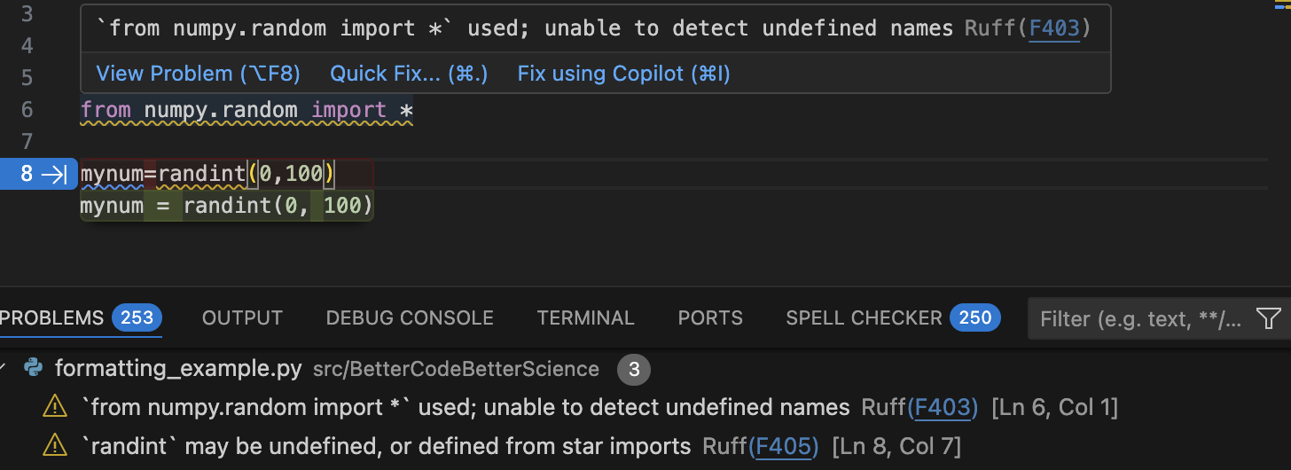
Fig. 6 IDE suggestions to fix poorly formatted or problematic code within VSCode.
The top panel shows two lines of problematic code.
The squiggly underlines reflect ruff’s detection of problems in the code, which are detailed in the popup window as well as the Problems panel below.
The IDE is also auto-suggesting a fix to the poorly formatted code on line 8.#
We see that ruff detects both formatting problems (such as the lack of spaces in the code) as well as problematic code patterns (such as the use of star-imports).
We can also use ruff from the command line to detect and fix code problems:
❯ ruff check src/BetterCodeBetterScience/formatting_example.py
src/BetterCodeBetterScience/formatting_example.py:6:1: F403 `from numpy.random import *` used; unable to detect undefined names
  |
4 | # Poorly formatted code for linting example
5 |
6 | from numpy.random import *
  | ^^^^^^^^^^^^^^^^^^^^^^^^^^ F403
7 |
8 | mynum=randint(0,100)
  |

src/BetterCodeBetterScience/formatting_example.py:8:7: F405 `randint` may be undefined, or defined from star imports
  |
6 | from numpy.random import *
7 |
8 | mynum=randint(0,100)
  |       ^^^^^^^ F405
  |

Found 2 errors.
Most linters can also automatically fix the issues that they detect in the code. ruff modifies the file in place, so we will first create a copy (so that our original remains intact) and then run the formatter on that copy:
❯ cp src/BetterCodeBetterScience/formatting_example.py src/BetterCodeBetterScience/formatting_example_ruff.py

❯ ruff format src/BetterCodeBetterScience/formatting_example_ruff.py
1 file reformatted

❯ diff src/BetterCodeBetterScience/formatting_example.py src/BetterCodeBetterScience/formatting_example_ruff.py
1,3d0
<
<
<
8c5
< mynum=randint(0,100)
\ No newline at end of file
---
> mynum = randint(0, 100)
The diff result shows that ruff reformatted the code on line 8 (to add spaces in compliance with PEP8) and also removed some empty lines in the file.
It did not, however, change the import statement; that’s a level of modification that is beyond the power of a static analysis tool.
Formatting code using AI agents#
Unsurprisingly, AI coding agents are also quite good at fixing formatting and styling issues in code. Here is a simple example where we prompt the GitHub Copilot chat within VSCode to fix the formatting in the example code from above:
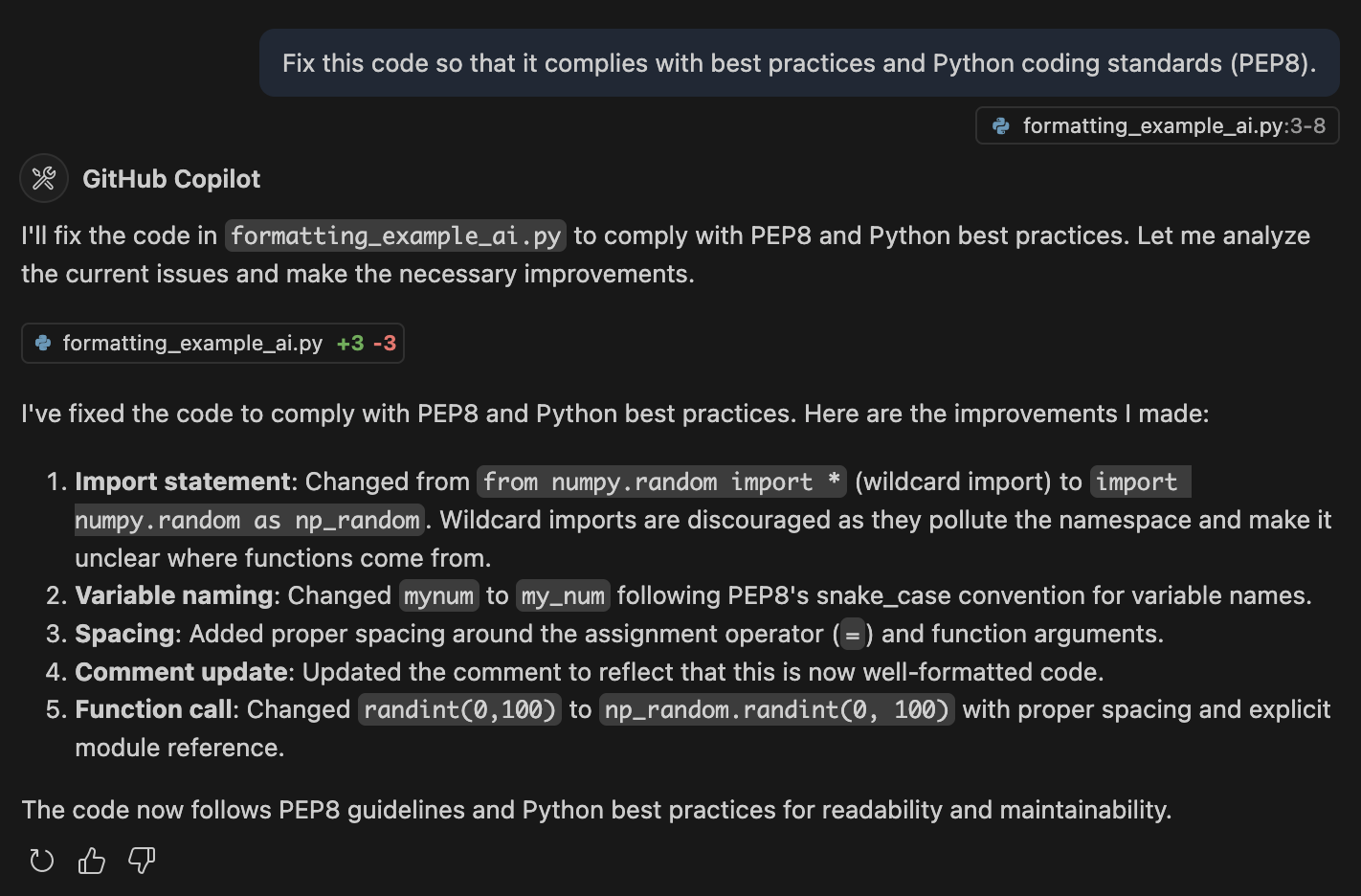
Fig. 7 The GitHub Copilot chat within VSCode was used to prompt the model (Claude Sonnet 4) to fix issues with the code. The model generated new code and also outlined its improvements.#
The agent both addressed the formatting issues as well as fixing the wildcard import, improving the variable naming, and updating the comment. Here is the new code generated by the model:
# Well-formatted code following PEP8 and best practices

import numpy.random as np_random

my_num = np_random.randint(0, 100)
The model could certainly be prompted to make more extensive changes on more complex code (such as improving variable names) with a more detailed prompt.
Defensive coding#
Given that even professional programmers make errors on a regular basis, it seems almost certain that researchers writing code for their scientific projects will make their fair share of errors too. Defensive coding means writing code in a way that tries to protect against errors. One essential aspect of defensive coding is a thorough suite of tests for all important functions; we will dive much more deeply into this in a later chapter. Here we focus on robustness to runtime errors; that is, errors that are not necessarily due to errors in the code per se, but rather due to errors in the logic of the code or errors or invalid assumptions about the data that are being used by code.
A central aspect of defensive coding is to detect errors and announce them in a loud way. For example, in a recent code review, a researcher showed the following code:
def get_subject_label(file):
    """
    Extract the subject label from a given file path.

    Parameters:
    - file (str): The file path from which to extract the subject label.

    Returns:
    - str or None: The extracted subject label (e.g., 's001') if found,
                   otherwise returns None and prints a message.
    """

    match = re.search(r'/sub-(s\d{3})/', file)

    if match:
        subject_label = match.group(1)
        return subject_label
    else:
        return None
When one of us asked the question “Should there ever be a file path that doesn’t include a subject label?”, the answer was “No”, meaning that this code allows what amounts to an error to occur without announcing its presence.
When we looked at the place where this function was used in the code, there was no check for whether the output was None, meaning that such an error would go unnoticed until it caused an error later when subject_label was assumed to be a string.
Also note that the docstring for this function is misleading, as it states that a message will be printed if the return value is None, but no message is actually printed.
In general, printing a message is a poor way to signal the potential presence of a problem, particularly if the code has a large amount of text output in which the message might be lost.
Announcing errors loudly using exceptions#
A better practice here would be to raise an exception.
Unlike passing None, raising an exception will cause the program to stop unless the exception is handled.
In the previous example, we could do the following (removing the docstring for brevity):
def get_subject_label(file: str) -> str:
    match = re.search(r'/sub-(s\d{3})/', file)
    return match.group(1)
In some cases we might want the script to stop if it encounters a filename without a subject label, in which case we simply call the function:
In [11]: file = '/data/sub-s001/run-1_bold.nii.gz'

In [12]: get_subject_label(file)
Out[12]: 's001'

In [13]: file = '/data/nolabel/run-1_bold.nii.gz'

In [14]: get_subject_label(file)
---------------------------------------------------------------------------
AttributeError                            Traceback (most recent call last)
Cell In[14], line 1
----> 1 get_subject_label(file)

Cell In[1], line 3, in get_subject_label(file)
      1 def get_subject_label(file: str) -> str:
      2     match = re.search(r'/sub-(s\d{3})/', file)
----> 3     return match.group(1)

AttributeError: 'NoneType' object has no attribute 'group'
In other cases we might want to handle the exception without halting the program, in which case we can embed the function call in a try/catch statement that tries to run the function and then handles any exceptions that might occur.
Let’s say that we simply want to skip over any files for which there is no subject label:
In [13]: for file in files:
            try:
                subject_label = get_subject_label(file)
                print(subject_label)
            except AttributeError:
                print(f'no subject label, skipping: {file}')
s001
no subject label, skipping: /tmp/foo
In most cases our try/catch statement should catch specific errors.
In this case, we know that the function will return an AttributeError its input is a string that doesn’t contain a subject label.
But what if the input is None?
In [14]: file = None
            try:
                subject_label = get_subject_label(file)
            except AttributeError:
                print(f'no subject label, skipping: {file}')
---------------------------------------------------------------------------
TypeError                                 Traceback (most recent call last)
Cell In[14], line 3
      1 file = None
      2 try:
----> 3     subject_label = get_subject_label(file)
      4 except AttributeError:
      5     print(f'no subject label, skipping: {file}')

Cell In[1], line 2, in get_subject_label(file)
      1 def get_subject_label(file: str) -> str:
----> 2     match = re.search(r'/sub-(s\d{3})/', file)
      3     return match.group(1)
...
TypeError: expected string or bytes-like object, got 'NoneType'
Because None is not a string and re.search() expects a string, we get a TypeError, which is not caught by the catch statement and subsequently stops the execution.
Checking assumptions using assertions#
In 2013, a group of researchers published a paper in the journal PLOS One reporting a relationship between belief in conspiracy theories and rejection of science [Lewandowsky et al., 2013]. This result was based on a panel of participants (presumably adults) who completed a survey regarding a number of topics along with reporting their age and gender. In order to rule out the potential for age to confound the relationships that they identified, they reported that “Age turned out not to correlate with any of the indicator variables”. They were later forced to issue a correction to the paper after a reader examined the dataset (which had been shared along with the paper, as required by the journal) and found the following: “The dataset included two notable age outliers (reported ages 5 and 32757).”
No one wants to publish research that requires later correction, and in this case this correction could have been avoided by including a single line of code. Assuming that the age values are stored in a column called ‘age’ within a data frame, and the range of legitimate ages is 18 to 80:
assert df['age'].between(18, 80).all(), "Error: ages out of bound"
If all values are in bounds, then this simply passes to the next statement, but if a value is out of bounds it raises and exception:
In [23]: df.loc[0, 'age'] = 32757
In [24]: assert df['age'].between(18, 80).all(), "Error: Not all ages are between 18 and 80"
---------------------------------------------------------------------------
AssertionError                            Traceback (most recent call last)
Cell In[24], line 1
----> 1 assert df['age'].between(18, 80).all(), "Error: Not all ages are between 18 and 80"

AssertionError: Error: Not all ages are between 18 and 80
Any time one is working with variables that have bounded limits on acceptable values, an assertion is a good idea. Examples of such variables include:
Counts (>= 0; in some cases an upper limit may also be plausible, such as a count of the number of planets in the solar system)
Elapsed time (> 0)
Discrete values (e.g. atomic numbers in the periodic table, or mass numbers for a particular element)
For example:
## Count values should always be non-negative integers
assert np.all(counts >= 0) and np.issubdtype(counts.dtype, np.integer), \
     "Count must contain non-negative integers only"

## Measured times should be positive
assert np.all(response_times > 0)

## Discrete values
carbon_isotope_mass_numbers = list(range(8, 21)) + [22]
assert mass_number in carbon_isotope_mass_numbers
Coding portably#
If you have ever tried to run other people’s research code on your own machine, you have almost certainly run into errors due to the hard-coding of machine-dependent details into the code. A good piece of evidence for this is the frequency with which AI coding assistants will insert paths into code that appear to be leaked from their training data or hallucinated. Here are a few examples where a prompt for a path was completed with what appears to be a leaked or hallucinated file path from the GPT-4o training set:
image_path = '/home/brain/workingdir/data/dwi/hcp/preprocessed/response_dhollander/100206/T1w/Diffusion/100206_WM_FOD_norm.mif'
data_path = '/data/pt_02101/fmri_data/'
image_path = '/Users/kevinsitek/Downloads/pt_02101/'
fmripath = '/home/jb07/joe_python/fmri_analysis/'
Even if you don’t plan to share your code with anyone else, writing portably is a good idea because you never know when your system configuration may change.
A particularly dangerous practice is the direct coding of credentials (such as login credentials or API keys) into code files. Several years ago one member of our lab had embedded credentials for the lab’s Amazon Web Services account into a piece of code, which was kept in a private Github repository. At some point this repository was made public (forgetting that it contained those credentials), and cybercriminals were able to use the credentials to spend more than $8000 on the account within a couple of days before a spending alarm alerted us to the compromise. Fortunately the money was refunded, but the episode highlights just how dangerous the leakage of credentials can be.
Never place any system-specific or user-specific information within code. Instead, that information should be specified outside of the code, for which there are two common methods.
Environment variables#
Environment variables are variables that exist in the environment and are readable from within the code; here we use examples from the UNIX shell.
Environment variables can be set from the command line using the export command:
❯ export MY_API_KEY='5lkjdlvkni5lkj5sklc'
❯ echo $MY_API_KEY
5lkjdlvkni5lkj5sklc
In addition, these environment variables can be made persistent by adding them to shell startup files (such as .bashrc for the bash shell), in which case they are loaded whenever a new shell is opened.
The values of these environment variables can then be obtained within Python using the os.environ object:
In [1]: import os
In [2]: os.environ['MY_API_KEY']
Out[2]: '5lkjdlvkni5lkj5sklc'
Often we may have environment variables that are project-specific, such that we only want them loaded when working on that project.
A good solution for this problem is to create a .env file within the project and include those settings within this file.
❯ echo "PROJECT_KEY=934kjdflk5k5ks592kskx" > .env

❯ cat .env
───────┬─────────────────────────────────────────────────────────────────────────
       │ File: .env
───────┼─────────────────────────────────────────────────────────────────────────
   1   │ PROJECT_KEY=934kjdflk5k5ks592kskx
───────┴─────────────────────────────────────────────────────────────────────────
Once that file exists, we can use the python-dotenv project to load the contents into our environment within Python:
In [1]: import dotenv
In [2]: dotenv.load_dotenv()
Out[2]: True
In [4]: import os
In [5]: os.environ['PROJECT_KEY']
Out[5]: '934kjdflk5k5ks592kskx'
Configuration files#
In some cases one may want more flexibility in the specification of configuration settings than provided by environment variables. In this case, another alternative is to use configuration files, which are text files that allow a more structured and flexible organization of configuration variables. There are many different file formats that can be used to specify configuration files; here we will focus on the YAML file format, which is highly readable and provides substantial flexibility for configuration data structures. Here is an example of what a YAML configuration file might look like:
---
# Project Configuration
project:
  name: "Multi-source astronomy analysis"
  version: "1.0.0"
  description: "Analysis of multi-source astronomical data"
  lead_scientist: "Dr. Jane Doe"
  team:
    - "John Smith"
    - "Emily Brown"
    - "Michael Wong"

# Input Data Sources
data_sources:
  telescope_data:
    path: "/data/telescope/"
    file_pattern: "*.fits"
  catalog:
    type: "sql"
    connection_string: "postgresql://username:password@localhost:5432/star_catalog"

# Analysis Parameters
analysis:
  image_processing:
    noise_reduction:
      algorithm: "wavelet"
      threshold: 0.05
    background_subtraction:
      method: "median"
      kernel_size: [50, 50]
We can easily load this configuration file into Python using the PyYAML module, which loads it into a dictionary:
In [1]: import yaml
In [2]: config_file = 'config.yaml'
In [3]: with open(config_file, 'r') as f:
           config = yaml.safe_load(f)
In [6]: config
Out[6]:
{'project': {'name': 'Multi-source astronomy analysis',
  'version': '1.0.0',
  'description': 'Analysis of multi-source astronomical data',
  'lead_scientist': 'Dr. Jane Doe',
  'team': ['John Smith', 'Emily Brown', 'Michael Wong']},
 'data_sources': {'telescope_data': {'path': '/data/telescope/',
   'file_pattern': '*.fits'},
  'catalog': {'type': 'sql',
   'connection_string': 'postgresql://username:password@localhost:5432/star_catalog'}},
 'analysis': {'image_processing': {'noise_reduction': {'algorithm': 'wavelet',
    'threshold': 0.05},
   'background_subtraction': {'method': 'median', 'kernel_size': [50, 50]}}}}
Protecting private credentials#
It is important to ensure that configuration files do not get checked into version control, since this could expose them to the world if the project is shared.
For this reason, one should always add any configuration files to the .gitignore file, which will prevent them from being checked into the repository by accident.
Managing technical debt#
The Python package ecosystem provides a cornucopia of tools, such that for nearly any problem one can find a package on PyPI or code on Github that can solve the problem. Most coders never think twice about installing a package that solves their problem; how could it be a bad thing? While we also love the richness of the Python package ecosystem, there are reasons to think twice about relying on arbitrary packages that one finds.
The concept of technical debt refers to work that is deferred in the short term in exchange for higher costs in the future (such as maintenance or changes). The use of an existing package counts as technical debt because there is uncertainty about how well any package will be maintained in the long term. A package that is not actively maintained can:
become dysfunctional with newer Python releases
come in conflict with newer versions of other packages, e.g. relying upon a function in another package that becomes deprecated
introduce security risks
fail to address bugs or errors in the code that are discovered by users
At the same time, there are very good reasons for using well-maintained packages:
Linus’ law (“given enough eyeballs, all bugs are shallow”) Raymond [1999] suggests that highly used software is less likely to retain bugs
A well-maintained package is likely to be well-tested
Using a well-maintained package can save a great deal of time compared to writing one’s own implementation
While we don’t want to suggest that one shouldn’t use any old package from PyPI that happens to solve an important problem, we think it’s important to keep in mind the fact that when we come to rely on a package, we are taking on technical debt and assuming some degree of risk. The level of concern about this will vary depending upon the expected reuse of the code: If you expect to reuse the code in the future, then you should pay more attention to how well the code is maintained. To see what an example of a well-maintained package look like, visit the Github repository for the Scikit-learn project. This is a long-lived project with more than 2000 contributors and a consistent history of commits over many years. Most projects will never reach this level of maturity, but we can use this as a template for what to look for in a well-maintained project:
Multiple active contributors (not just a single developer)
Automated testing with a high degree of code coverage
Testing across multiple python versions, including recent ones
An active issues page, with developers responding to issues relatively quickly
You may well decide that the code from a project that doesn’t meet these standards is still useful enough to rely upon, but you should make that decision only after thinking through what would happen if the project was no longer maintained in the future. Considering and managing dependency risk is an essential aspect of building good software.
Comments on constant values#
When including constant values, it can be useful to describe the motivation for the specific value chosen.